With xlCompare, you can get a list of missing rows in an Excel spreadsheet in just a few clicks - quickly and easily. We'll show you how to get the result without using complicated VLOOKUP or XLOOKUP formulas.
Every time you receive a new spreadsheet with customer or product data, you need to verify that all records are correct and complete.
A common approach is to compare the file against a template or against the same spreadsheet from the previous month and identify all rows that do not match.
For example, you may need to verify that every item was correctly added to a price list containing 10,000 products.
Tasks like these should not be done manually - the risk of human error is too high. The online application xlCompare automates this process and solves the problem in seconds.
Below, we'll show you how to compare two Excel price lists and save the rows that are missing from the other list.
Drag and Drop Two Files onto This Page
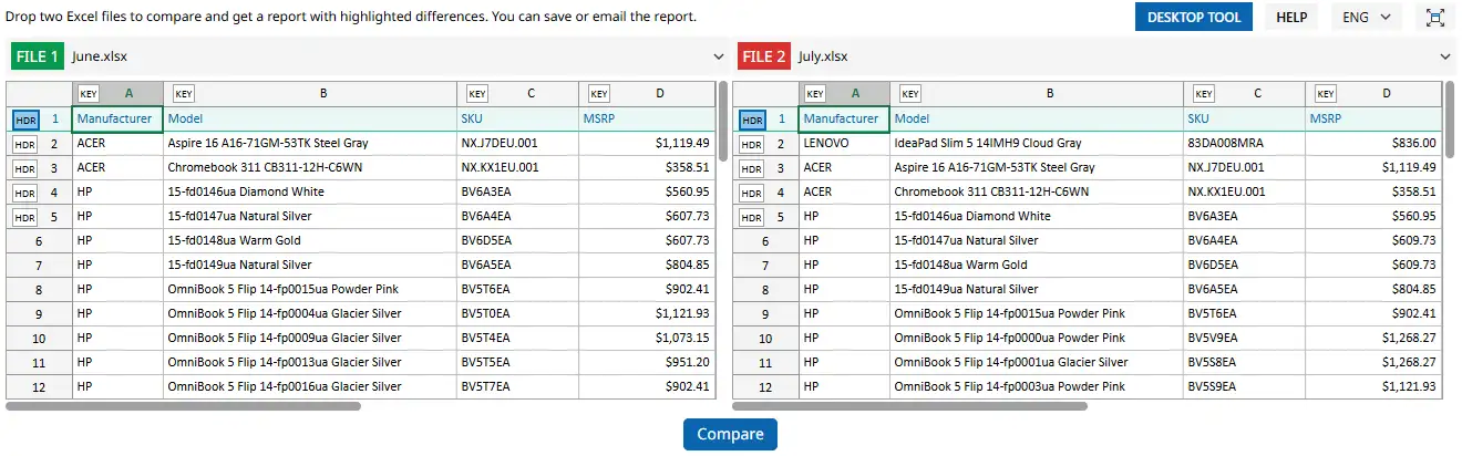
To get started, drag and drop two files from File Explorer onto this page. Place one file in the left panel and the other in the right panel.
You can also paste data directly into the tables using the clipboard. This option is especially useful if your spreadsheets are stored in Google Sheets or use a format other than XLSX or CSV.
In our example, it looks like this:
Specify the Header Row and Key Column
You can skip this step if your table does not contain a header row. However, it is important to get accurate results. The header row gives xlCompare the field names from your table, while the key column tells the application which field should be used to match rows between the two tables.
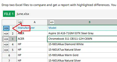
How to Select the Header Row
Click the HDR marker next to the row number. The selected row will be highlighted in blue.
In our example, the first row in each table is the header row.
What if there is no header row? Simply skip this step - it will not affect the comparison result.
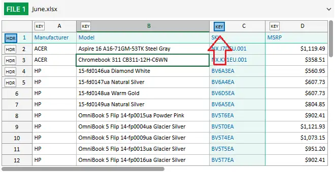
How to Specify the Key Column
Click the KEY marker in the column header. The selected column will be highlighted in blue.
In our example, we use the SKU column as the key field. This field uniquely identifies each row in the table.
In more advanced cases, the key can consist of multiple fields, such as first name and last name.
What if you are not sure which field to use as the key? Just skip this step. In that case, xlCompare will use a different algorithm to find differences between the tables.
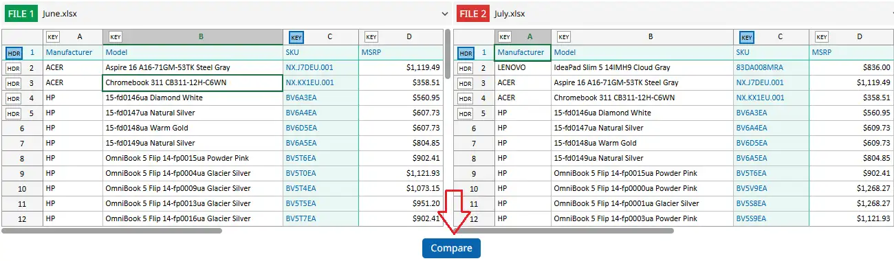
Compare the Two Tables
Click the Compare button located below the two tables to run the comparison and instantly see the results on the screen.
All differences between the two tables will be highlighted with colors for easy review.
Result is the following:
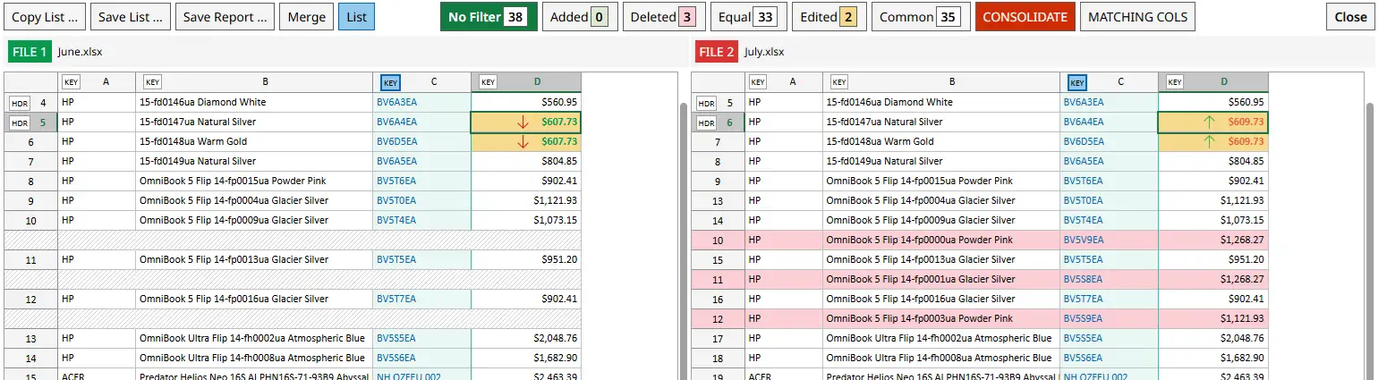
Get a List of Non-Matching Rows
Above the comparison report, you will see the Legend, which displays the number of matching and different rows.
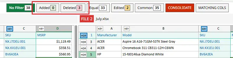
Select Added, and xlCompare will display only the rows whose SKU does not exist in the right-hand list. These rows are highlighted in green.
If you select Deleted, xlCompare will display the rows that are missing from the right-hand file. These rows are highlighted in red.
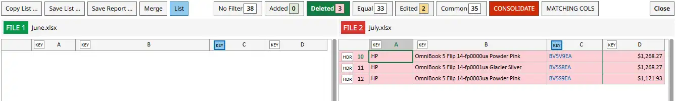
That's exactly what we need.
Save the Resulting List
The online version of xlCompare does not save files directly to your disk. Instead, it allows you to copy the resulting table and paste it into a new Excel file or Google Sheets document.
This is a simple and familiar way to transfer data between spreadsheets - even for beginners.
Right-click anywhere inside one of the tables.
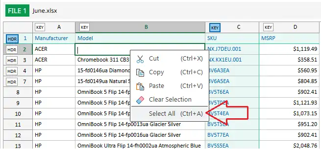
Click Select All in the context menu.
Right-click again and select Copy.
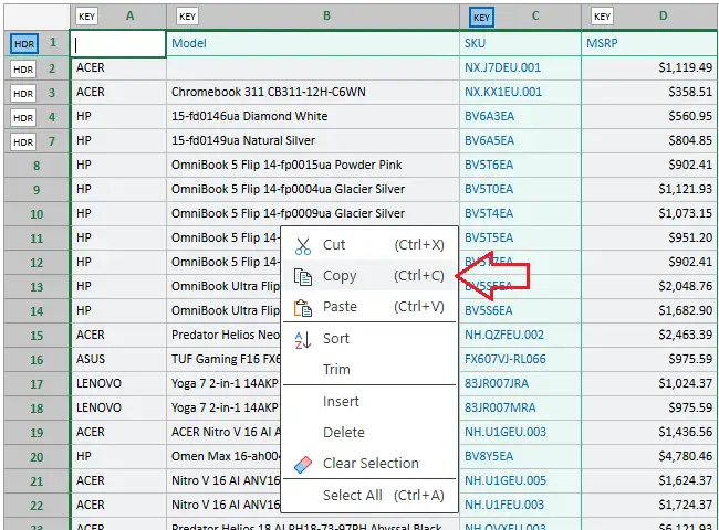
Done! The selected data is now stored in your clipboard.
You can now paste it directly into Microsoft Excel or Google Sheets.
You can also use keyboard shortcuts instead of the context menu:
- Ctrl+A - Select All
- Ctrl+C - Copy
Conclusion
As you can see, the entire task can be completed in just a few clicks.
Even if you are highly experienced with Excel formulas, functions, and advanced features, getting the result with 5–6 mouse clicks is faster and easier.
